Saturday, November 11, 2017

Make a Money In 'N Out Spreadsheet With Your Teen

Teen With Money In N Out Pie Charts

For many kids, money can be a bit too easy come, easy go — especially in today’s digital world.

But tracking and categorizing money thoughtfully will always be a key life skill. Dollars deserve a purpose whether digital or not. So how do we get our kids to be more mindful of money as it ebbs and flows?

Build a Money In ’N Out Spreadsheet with your child. It’s a simple tool for pinpointing the sources for money coming in and the purposes for money going out.
Here’s a recipe I used with my son in college:

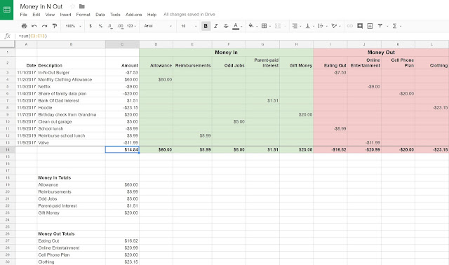
  1. Import last month’s transactions. Most prepaid cards or bank cards have a way to export transactions, so this step is often just a quick cut and paste. If your teen uses cash, then have her manually enter every transaction in the spreadsheet for the current month.
  2. Add “Money In” columns. Sit down together and figure out the main types of income. Create columns for each. In our case, money coming in was either:
  3. Add “Money Out” columns. For money coming out, let you child suggest the key categories of spending as you browse the transactions together. Less is more here, so steer it toward high level groupings. We ended up with:
    • eating out,
    • eating in,
    • health,
    • gaming, and
    • phone.
    The right categories will depend upon what your child is responsible for purchasing directly. If your teen has very few transactions, that’s probably a sign you need to relinquish more purchasing responsibility. Either create some appropriate budget-based allowances or use a reimbursement strategy, or both.
  4. Copy the transaction amount into the right in or out column. For each transaction row, copy the amount into the appropriate income or spending column. In rare cases, you may need to split the amount between spending columns. But if you’re doing that a lot, your categories are probably too granular. Keep it simple — like the In-N-Out menu.
  5. Sum up the totals. Add a final row that sums up the amount column, the income columns, and the spending columns. The sum of the amount column will indicate the net change for the month. If it’s negative, more was spent than earned during the period.
  6. Make in ’n out pie charts. Create an “in” pie chart for the income totals, and an “out” pie chart for the spending totals. Any surprises?

  7. Have a non-judgmental discussion. Here’s where you want to be long on listening and short on lecturing. Let your child make the observations. Offer constructive alternatives, like maybe a parent bounty for taking a bag lunch instead of eating out.

I created a Money In N Out spreadsheet template in Google Docs that you can copy and adjust to your liking. Check it out here.

Try the exercise with your teen, and see if it takes the money coming and going in a more mindful direction.


Want to turn these tips into action? Check out FamZoo.com.

Thursday, November 2, 2017

Plot Your Longest Market Losing Streak Since High School

Boy making loser hand gesture.

My longest market losing streak since high school is pretty epic.

If I had invested $5,000 in the S&P 500 on January 1, 2000, it would have been worth less than that for 12 years in a row. Ouch.

But, as Tom Petty said, “Even the losers get lucky sometimes.” Especially if they wait long enough in the market. By October 2017, that original $5,000 investment would have turned into $8,976.49. Not too shabby!

But, remember, Tom also said, “The waiting is the hardest part.

Here’s a simple spreadsheet exercise you can use to convince your teens (or your spouse or even yourself) to invest patiently in the market — even when the going gets tough.

Plot your hypothetical market winning and losing streaks dating all the way back to high school.

My spreadsheet shows what would happen to an investment in the S&P 500 from a given year til now for every year since my freshman year in high school. That was 1976 in case you were wondering.

This is one of those rare times where the older you are, the better it gets. So, if you’re a young parent, you may want to use grandpa or grandma as a reference point instead.

Here’s how to make a spreadsheet like mine in Google Docs:

  1. Find a source of historical S&P 500 data. I found mine here at multpl.com.
  2. Add a price column for every year since the beginning of high school. Pro tip: I was able to do this very quickly by copying the data table entries on multpl.com from the top down to the 1976 entry, pasting them vertically into a temporary sheet, sorting the data by date descending, selecting the sorted data, creating a new sheet, and using Edit > Paste Special > Paste Transposed to lay out the data horizontally across the sheet. Beats the heck out of typing!
  3. Define an annual contribution. Insert a couple rows up at the top, enter an amount for your fixed annual contribution size, and use Data > Named Ranges... to assign the amount to a name (like “contrib”). Then you can use that name in your formulas.
  4. Enter rows representing the investment performance for each year. Find the column for the starting year, and enter the initial contribution amount as the formula “=contrib”.

    Fill out the remaining columns with the formula that calculates the value of the investment a year later by using the historical price data up above. My price data is in row 4, so the formula for the first anniversary of my initial investment in cell B5 looks like: “=A5+((B$4-A$4)/A$4)*A5”.

    The cool thing is I can now just select that cell along with all the cells to its right and type Control-r to copy the formula across the row. Now I’ll see the value of the initial investment each year from inception to present day.

    I repeat this for each successive row starting one column over to the right each time until I get to the current year. At the end, it looks like an upside down ramp.

  5. Add conditional formatting to call out winning and losing years. A winning year is when the current cell’s value is greater than the initial contribution. Make those cells green. Otherwise, make the cell red to mark a losing year. You can create the conditional formatting rules from the Format > Conditional formatting... menu entry.
  6. Add running totals across the bottom. Summing the rows for each column will give the total value of all investments for each year across the bottom. I like to compare that with what would happen if I had just kept the contributions in cash the whole time.

Check out my win/loss plot.

Step back and admire all that green. It dominates. And, at the moment, there isn’t a single row that hasn’t turned green ultimately.

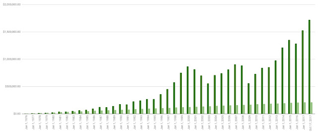
At the bottom right, compare the total ending value of the investments versus just stashing the same contribution in cash year after year. In my case: $1,719,627.25 vs $210,000.00.

Wow.

By the way, I’m ignoring dividends and expenses to keep things simple. With or without them, the point remains loud and clear: Dollar cost averaging plus low cost index funds for the win!

Despite an occasional epic losing streak, your simple market win/loss spreadsheet will prove to your kids that patient, consistent investing kicks cash’s backside over the long run.

All the more reason to start your teen’s Family 401(k) asap!


Want to turn these tips into action? Check out FamZoo.com.